Interactive Benchmarking

IB^®

User Guide and Help Screen

ver. 2.8

Sept, 2012

Peter Bogetoft

pb@ibensoft.com

· Note: Some of the facilities described in this manual may not be available to you since they depend on user rights. Also, a few of the facilities (like Survey) is only available in the Web-based version and not in the Windows based version.

Content

General information on Interactive Benchmarking IB®

Login

Select Model: Predefined Model

Select Model: Selfdefined Model

Select Units: My Unit

Select Units: Merge

Select Units: Potential Peers

Scenario / Survey

KPI

Benchmark

Peer Units

Sector Analysis

Dynamic

Reports

Data: Data

Data: Models

Data: Setup

General information on Interactive Benchmarking IB^®

The idea

Interactive Benchmarking IB^® is an interactive computer program that organizes and analyzes data with the objective of improving performance. It combines state-of-the-art benchmarking theory, decision support methods and computer software to identify appropriate role models and useful performance standards.

Background

In the last decades, theorists and practitioners have devoted a lot of interest to benchmarking and relative performance evaluations. Most analyses, however, rely on a series of presumptions. The evaluated units may question these assumptions and hereby the relevance of the results. Moreover, they may ask a series of what-if questions. It is therefore important to tailor the benchmarking to the specific application and users.

Tailored benchmarking

To allow tailored benchmarks, we have embedded state-of-the-art methods in a easy-to-use software. IB hereby offers a benchmarking environment rather than a benchmarking report based on more less arbitrary assumptions of the analyst. A User interacts directly with a computer system to make the analyses reflect its specific focus, conditions, mission and aspirations.

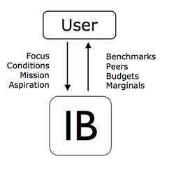
Focus: The user selects a focus (Model) for the analysis. The focus can be short run or long run, and it can involve the whole firm or some parts of its. The benchmarking system comes preloaded with relevant models but it also allows the user the possibility to develop its own focus.

Conditions: The models are defined to capture the relevant conditions. However, the user can make further presumptions about itself (MyUnit) and its relevant comparators (Potential Peers). The evaluated unit can be a realized one, a budgeted one, a merged firm etc. Similarly, comparison with some of the others can be excluded via filters on the allowed peers. The User may for example only be interested in comparisons with local firms of similar size.

Mission: The specific mission or strategy of the user can be further specified by defining search directions. How keen is the user to save on the different inputs (resources) and to expand the different outputs (products and services) ?

Aspirations: The aspiration level and performance of others can be examined as well. Although best practice is of particular interest, the user may strive for less, e.g. 25% best practice. Likewise, the user may be interested in how well the others do with respect to the same mission.

Other general features

Easy to use: The controls of the interactive benchmarking process are simple and intuitive. Also, an extensive help system assists the user in the (less likely) case of doubt.

Applicable: The results are directly applicable in business decisions. IB offers a learning lab for managers based on complex multiple inputs multiple output relationships derived from actual practices. Also, it calculates plans and budgets and peers to learn from in the implementation. It informs the user of marginal costs, substitution between production factors and trade-off between services. It allow the user to predict synergies from mergers and much more.

Research team: Behind the scene, the program involves best practice in performance evaluation and computer technology. It is developed by a team headed by Professor Peter Bogetoft, a leading international scholar in performance evaluation, the author of more than 50 peer review articles and books, and a consultant on numerous benchmarking exercises throughout the world.

Technical details: For more on the theory and the mathematical and statistical methods, contact the developers at pb@ibensoft.com.

Login

Login

The login tab requires a login username and a password. This determines the tabs you can see, the facilities you can use in the different tabs, and the other choices you can make in the model.

“?”

On the top right of the screen, the “?” links to the help system. The help topics are specific to the tab that you are looking at when you activate it.

Normal IB session flows

The normal usage of Interactive Benchmarking IB^® will take you sequentially from the left to the right tab

· At any time, you can jump back to a former tab and change you choice. You can for example change the model used to analyze performance or change the unit you are analyzing.

· If you insert a new data file as explained above, you are forced to start back at the login screen.

· In a session, the tabs will light up when they are available. Your can for example NOT use Benchmark before you have selected a model and a unit to analyze.

IB general controls

There are many possibilities to alter the look of the windows. The possibilities and handles are intuitive and based on standard procedures in Windows. Drag rows, columns and windows.

How to update IB-Win

· Whenever you start a session, IB will check if you have Internet access. If so, it will look for updates.

· If an update exists, you can choose to install it

· If you later regret the updating, you can go back to earlier versions of the program via “add and remove programs” in Windows control panel.

Select Model: Predefined Model

Select Model: Predefined Model

· You can see the predefined models in the Select Predefined model sub-tab.

· When you mark a predefined model, a description becomes available at the lower part of the screen.

· The predefined models have been proposed by the provider and offer a starting point for the user. The user can define alternative models in the Selfdefined Model tab.

A model

A model is defined by inputs, outputs and context variables.

· The inputs represent resources used, costs etc.

· The outputs represent the products or services generated.

· The context variables are non-controllable conditions that may either ease or complicate the transformation of inputs into outputs.

A model defines one focus for the analysis. It can be short run or long run, and it can involve the whole firm or some parts of it, perhaps a process.

Select Model: Selfdefined Model

Select Model: Selfdefined Model

In the Select Selfdefined Model tab, you can define your own model by specifying

· Inputs (I), i.e. resources and costs used

· Outputs (O), i.e. the products or services generated

You can choose from any of the variables initially indicated as

· Read-only (R), variables, i.e. variables you could have use

Sample size

As the Inputs and Outputs are chosen, the program calculates the relevant (sub-) Sample, i.e. the units with data on all the chosen variables.

Locked variables

The table also gives a series of

· Locked variables (L). They cannot be used as inputs or outputs, e.g. because they contain non-numerical information.

Usage of other variables

The Read-only (R) variables that are not used directly as Inputs or Outputs and the Locked (L) variables (if it makes sense) can be used in the delineation of relevant comparators in the Select Units: Potential Peers tab. Also, they can be used as possible explanatory variables of performance in the Sector Analysis: Show graphs: Second stage analysis.

Estimation approach

The model specification (Inputs and Outputs) defines the focus of the model. To turn it into a genuine model, we must also determine the relationship between the variables. The estimation approach used for self-defined models is that of minimal extrapolation. The idea of the corresponding so-called non-parametric FDH and DEA approaches is to extrapolate the least from data – to find the closest possible approximation of the actual data.

It is also possible to use models estimated using parametric (PAR) econometric approaches like SFA. They must be determined using econometric skills and then be defined in the data sheet. PAR is therefore not an option in the Select Model: Selfdefined Model tab – only in the

Select Model: Predefined Model tab.

Return to scale

You must also specify the return to scale. This gives your a priori beliefs about the effects of increasing and decreasing the scale of operations. The questions is if more inputs are required per output bundle as the scale of operation gets larger (large scale disadvantages) or smaller (small scale disadvantages).

In other words, if we increase the inputs with some percentage but do not believe that the outputs can be increased with the same percentage, then we believe in disadvantages of being larger. Likewise, if we decrease the input with some percentage and believe that the outputs will fall with a larger percentage, then we believe in disadvantages of being small. A common reason to expect difficulties of a too large operation is increased coordination and communication tasks. Similarly, a common reason to expect difficulties of a too small operation is the presence of fixed costs or the need to have effective specialization.

Possible Returns to scale

There are six possible settings for the Return to scale:

· Constant Return to Scale (CRS) means that we do not believe there to be significant disadvantage of being small or large

· Decreasing Return to Scale (DRS) means that there may be disadvantages of being large but no disadvantages of being small

· Increasing Return to Scale (IRS) means that there may be disadvantages of being small but no disadvantages of being large

· Variable Return to Scale (VRS) means that there are likely disadvantages of being to too small and too large.

· Extended Free Disposability Hull (FHD+) means that we no ex ante assumptions about the impact on size except some limited local return to scale for scaling factors between L and H

· Additivity (ADD) mean that one can always repeat what others have done, and one can therefore also do what any combination of other have done by letting the parts operate as independent entities

If you later regret you’re a priori assumptions about Return to scale, you can change the assumption on the run in the Benchmark tab, cf. below

Name and load model

· Before you can continue, you must also name the model and provide a description.

· If you have defined your own model in a previous session, you can load it here using the Load button.

Select Units: My Unit

In My Unit you select the unit you want to analyze.

Existing Unit

· You can choose to analyze an Exiting unit

· Its values of the Inputs (I) and Outputs (O) then shows up in the window below.

Selfdefined

· You can also choose to define your own unit, Selfdefined.

· You can give it a name as you like

· You must put in the relevant values for the Inputs and Outputs in the table

· If your Selfdefined unit resembles an existing one, you can mark this first and them simply modify the numbers of the existing unit.

Use of Selfdefined unit

The option to define you own unit is useful in many cases, including analyses of the possibilities to make improvements

· of an exiting budget

· in an average year

· after already planned changes

Use of variable transformations

In some applications there it is convenient to allow different representations of the inputs and outputs. In a school benchmark, we might for example want the performances of all school to be re-calculated as if they all had student with socio-economic background like the specific school we are investigating. Similarly, we might be interested in firms’ performances in different economic scenarios, say with increasing interests rates and with decreasing interest rates. The necessary recalculations of the data points can be done using variable transformation Vtrans. In the My Unit tab. Vtrans is available when such transformations are defined in a Vtrans sheet of the Data xls sheet.

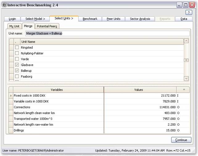
Select Units: Merge

In Merge you can analyze the performance of a potential merger of two or more units.

Procedure

You indicate which of the existing units you would like to be included in the potential merger. Interactive Benchmarking IB^® then names this unit as

“Candidate1+Candidate2+…+CandidateK”

and their combined resource usage (sum of their pre-merger inputs) as inputs and their combined production (sum of their pre-merger outputs) as outputs. 

This entity can then be analyzed like any other Selfdefined unit. High saving potentials compared to the individuals involved in the merger suggest large potential gains from the merger. 

Caveats

In some models the simple addition of inputs and outputs that the merger option facilitates may not make sense. An example of this is when some inputs or outputs are proportions or fractions, e.g. the fraction of products being of high quality. To handle such cases one should either redefine the products to be units that can naturally be added; for example units of high and units of low quality. Or one must calculate the resulting fraction of the merged entity by weighing together the fractions for the individual units and then using the resulting values in the Select Units: My Unit tab.

Interpretation

In the interpretation, the combined inputs and outputs would result if the merged entity was operated in a fully decentralized manner with each of the pre-merger units acting as independent “divisions” at a level of efficiency similar to the past.

In terms of interpretations, we note that the combined inputs and outputs would result if the merged entity was operated in a fully decentralized manner with each of the pre-merger units acting as independent “divisions” at a level of efficiency similar to the past..

The potential improvements of the merged unit “Candidate1+Candidate2+… +CandidateK” can therefore be interpreted as what can be gained by learning best practices and by optimally exploiting the synergy effects among the included entities. The latter can furthermore be decomposed in a mix and a scale component. A formal decomposition into these effects and organizational interpretations as developed in Bogetoft, P. and D. Wang, Estimating the Potential Gains from Mergers, Journal of Productivity Analysis, 23, pp. 145-171, 2005, and implemented in the

Aspiration

The aspiration Asp.% pull down allow user to benchmark against performance standards that are x% above or below best realized practice.

If for example the aspiration level is set to -10%, it means that we strive only to be 10% below the best practice production frontier. This is also useful to take into account expected productivity improvement, eg a 2% percent improvement in productivity over the next year can be accounted for by contemplating a 2% aspiration level based on today’s data.

The aspiration level is in absolute terms. If user’s aspiration is to be for example among the 10% best performing firms, a sector analysis can be done based on an output proportional direction, and the top 10% fractile of the efficiency distribution can be read off the distribution graph. If this is for example 1.17, it means that an absolute aspiration level of 17% corresponds to the top 10% performance.

The aspiration level has no impact in models without any outputs.

Merger analysispop-up in the Benchmarking tab.

Horizontal or vertical mergers

The merger option in Interactive Benchmarking IB^® is directly applicable to horizontal mergers, i.e. the integration of units producing the same types of services (outputs) using the same types of resources (inputs).

A vertical merger occur when an upstream firm integrates with a downstream firm. The upstream firm produces services (intermediate products) that are used as resources in the downstream firm. Vertical mergers can also be evaluated by Interactive Benchmarking IB^®. To do so you shall model both production processes as special cases of a combined model. In particular, this can be done by thinking in terms of netputs, i.e. inputs as negative netputs, and outputs as positive netputs. This approach is also applicable for more advanced networks where some of the outputs of the upstream units are final products while others are intermediate products serving also as inputs for the downstream unit. For more vertical mergers and networks, see

Bogetoft, P., Efficiency Gains from Mergers in the Health Care Sector, Part B: Modelling and Part C: Implementation, Research Papers 2008:07 and 2008:08, NZa, The Netherlands.

Select Units: Potential Peers

In Potential Peers you can restrict the units you want “My Unit” to be compared to. They are the ones defining the best practice against which you want to compare My Unit.

Be aware

The benchmarking procedure itself will usually generate reasonable comparators. In fact, this is a good indication that the model is reasonably specified.

Peers window

· The right Peers window gives the potential units that are left for comparisons.

· Individual units can be excluded by un-checking them - and you can undo the picking if you regret. The picking can also be done from the Benchmark tab.

Potential peers left and Included

· Potential peers left is the size of the comparator base. It depends on the model selected and the general Filters that are active in the left part of the Potential Peers tab, c.f. below.

· Included gives the number Potential Peers minus the individually Picked (excluded) units

Filters

· To define the relevant comparison group you can also use Filters. They are defined in the upper left part of the Potential Peers tab.

· You define a filter by using standard logical expressions.

· Pressing + a new condition is generated. Moving the curser over the line, you get the possible choices in each position

· In the example, we only want to compare with units with “Kapital” at least 2000 and with a name starting with a.

· Pressing Define activates the filter

· HINT: By scrolling right in the Peers window to the right, you can see the values of the different variables in the different units. This is useful to get an idea of the relevance of alternative filters.

Groups

Interesting Potential Peer Groups defined via a filter or by individually checking the Units in the right hand side list of firms can be saved as Peer Groups using the Save group button.

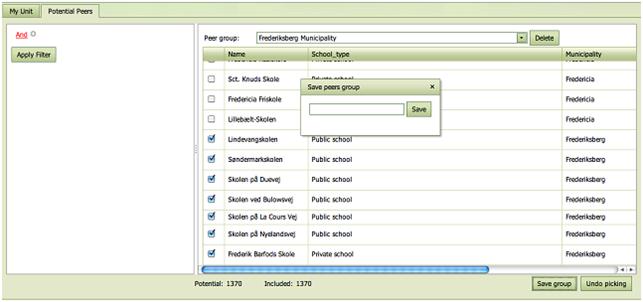
They are given a name by the user or have already been defined and named by the data provider.

The Groups are useful in the analysis since user may want to restrict the group of comparators.

Stock of filters in IB-Win

· In the lower left window, you find the stock of filters that you have defined.

· The active ones are checked. It can be deactivated by unchecking and (re) activated by checking its box.

· The Deactivate all allows this to be simplified when many filters are combined.

Edit and Delete

· An already defined filter can be edited. Pressing Edit, the filter moves into the definition window and can be adjusted.

· A given filter can also be deleted by using the Delete button.

Show

· Using Show, you can change what you see in this tab.

Usage of Filters and Picking

The possibility to make specific restrictions on the analyzed units is useful in many situations. Classical applications include

· Nominal variable – e.g. coops or investor owned companies, liberal or conservative regions, east or vest etc – may cal for a splitting of the sample to make the comparisons more interests. A cooperative may for example be more interested in comparisons with other cooperatives than with comparisons with investor owned firms.

· Ordinal variable – e.g. low quality, medium and high quality, complicated or simple cases etc – may likewise call for a splitting of the sample. It will typically be the case that the simple products of low quality produced under easy conditions can be benchmarked to similar products as well as to more complicated products of higher quality produced under more difficult conditions. The latter however cannot reasonably be compared to the former.

· Time variables – e.g. data from different years - may also be interesting as a filter parameter. E.g. to evaluate progress compared to a fixed performance standard, say last years best practice.

Scenario/Survey

IB-Web can be used not only to benchmark based on existing data but also to introduce, validate, benchmark and collect new data.

The facility can also be – and most commonly is – used to define alternative scenario and hereby alternative versions of MyUnit that can be benchmarked as part of a planning exercise. Instead of introducing new values of the variables directly as a self-defined unit, the Scenario can help calculate and define some or all of the variables in the model.

The Scenario / Survey is conditioned on the selected model, i.e. different Scenario / Survey templates can be affiliated with different models. The scenario tab will become visible whenever a Scenario is affiliated with chosen model. The Scenario / Survey can be accessed directly or via the link on the My Unit sub-tab. In Scenario applications it is convenient to start from a given unit since values that are not provided by the scenario will then be inherited from that unit.

As a direct user you can

· Provide numbers in any of the cells of the Scenario / Survey

· Leave the default values in the survey if they are appropriate to you

· Update the survey. This will make IB calculate any derived values (results) shown to the right of the answer cells and as well as any validation warnings shown in red to the right of the derived values (results).

· Save the information such that it can be used in the present and later IB sessions. Here you must indicate for which Unit you have provided information. You can also introduce a new name for the unit here.

· Send information to the survey provider.

An example is shown below. Here we save a version of Center 1 where the cost allocation is altered.

The definition of Scenarios / Surveys are done in tab of the Data: Data work book called Scenario_1, Scenario_2, etc.

KPI

KPI = Key Performance Indicators

Traditional benchmarking makes use of a selection of key performance indicators. This tab allows the user to explore these one by one and to also get a holistic picture of several KPIs.

In this help screen we will explain in particular

· How to choose a KPI

· Summary statistics

· A single KPI evaluation of MyUnit

· Multiple KPIs evaluation of MyUnit

· Zooming

· Trimming

· Printing

How to choose a KPI

The KPI must be predefined in the data set, and the user can select one KPI to analyze via a scroll down menu.

It is possible to select KPIs on which there is no data for MyUnit.

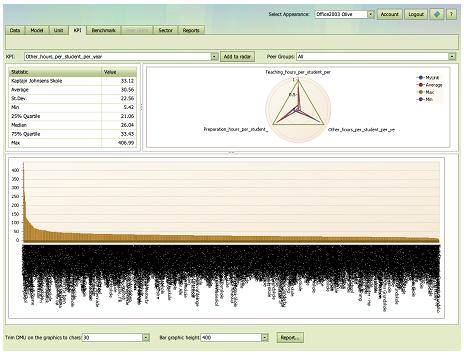
Summary statistics

The top left table provides summary statistics for the KPI selected and displayed just above the table. The Units that these summary statistics cover are those delineated in the Potential Peers tab. If no filters have been introduced here and if no units have been deselected in the Benchmark tab, the sample are all the Units for which the data set contains information about the KPI.

The summary statics provide information about the KPI in the group of Potential Peers on

· MyUnit, i.e. value of the KPI for MyUnit

· Average value, i.e. the (un-weighted) KPI value around which actual KPIs varies

· St.Dev (standard deviation), i.e. a measure of the spread in the KPIs

· Min (minimum), i.e. the smallest KPI value in the sample

· 25% Quartile, i.e. the KPI value that 25% of the units are below and 75% are above

· Median, i.e. the KPI value that 50% of the units are below and 50% are above

· 75% Quartile, i.e. the KPI that 75% of the units are below and 25% are above

· Max (maximum), i.e. the largest KPI value in the sample.

A single KPI evaluation of MyUnit

In the bar chart graph below the table, we depict the value of the KPI for all Potential Peers. The units are ordered such that low KPIs are to the left and high values are to the right. MyUnit is, if we have a value for this, emphasized as a red bar.

Multiple KPIs evaluation of MyUnit

To get an overview of several KPIs simultaneously, user can construct a radar diagram. The dimensions in the radar are picked by the user sequentially by selecting a KPI and then pressing “Add to Radar”. In each dimension, the radar then shows not only the minimal and the maximal value of the KPI in question, but also the average value in the sample and the value of MyUnit.

The radar is constructed relative to the maximal value in each dimension. Hence, a value of say 0.5 in a given direction means 50% of the maximal value. In the illustration above, we see that MyUnit is approx 0.3 in the Operating costs dimension. This corresponds to what can be seen in the table to the left, since the value of MyUnit divided by the value of Max, 43000/144117, is approximately 0.3.

Zoom and dragging

The bar chart can be examined in more details by scrolling and zooming.

The user can scroll the mouse wheel to zoom in and out of a chart's diagram in the same way one can zoom in commonly used Windows applications.

To activate the zoom function and make the selection more precise, simply press the SHIFT key. The mouse pointer is changed to a magnifying glass. Now select a region on a chart using the left mouse button.

Once the graph has been zoomed, a user can also click a chart's diagram and drag it left and right and up and down by using the hand symbol

Trimming

The names of the units and the KPIs in some data sets may be rather long and the bar chart and the radar chart may for this reason not look their best. To handle such cases, user can using Trim in the lower right corner. It limits the numbers of characters used.

Bar heights

Bar heights can also be trimmed to have appropriate heights using the Bar height at the bottom of the screen.

Groups

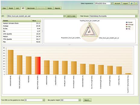
The comparison groups can be controlled via the Group scroll down at the top right of the page. The available groups are defined in the Select Units: Potential Peers tab or they may have been pre-defined in the Data:PeerGroups set.

Using an appropriate group is often useful the make the KPI statistics more relevant and to trim the graphics as illustrated below where the first involves all Units and the second only the schools in the same municipality as the school being analyzed.

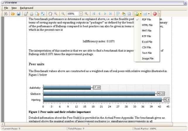
Reporting

You can collect interesting results using the Report facility. A pop-up window is hereby activated in which user can name the report and decide which part of the KPI screen to include in the report.

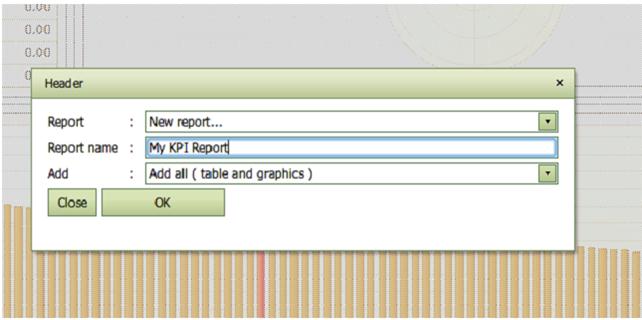
User can later extend the report by adding tables and diagrams for other specific KPIs

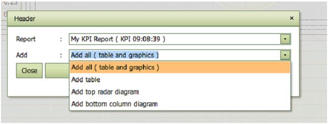
The report can at any time be shown and downloaded in different formats in the Reports tab.

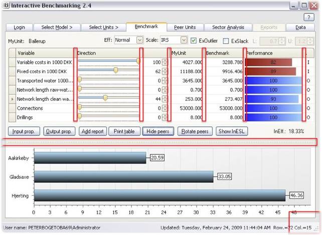
Benchmark

Benchmark is the central tab. It takes My Unit and compares it against a combination of other units and allows you to control the comparisons in a number of ways.

In this help screen we will explain in particular the

· Benchmark table

· Benchmark graphics

· Simultaneous improvements

· Improvement directions

· Proportional contractions and expansions

· MyUnit

· Peer Groups

· Show peers

· Eliminate specific peers

· InEfficiency Step Ladder

· Scale (and estimation principle)

· Efficiency

· Exclude slack

· Exclude outliers

· Aspiration

· Merger analysis

· Add report

· Print table

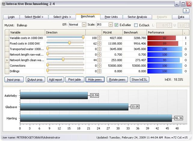
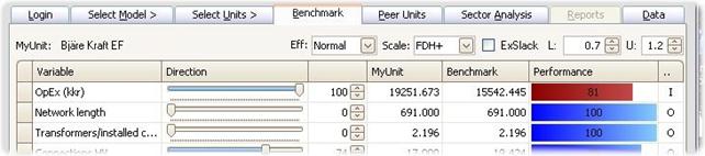
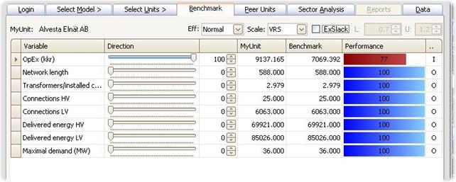
Benchmark table

The table compares the values of My Unit given in Present values, against the values of a Potential Peer or a combination of Potential Peers as given in Benchmark values. This is like comparing a realized account or development against a budget or a plan.

The Benchmark is constructed by considering all Potential Peers and a class of possible combinations hereof. Among the resulting (typically infinite number of possible comparators) the program picks the one that offers the largest potential improvement in performance of My Unit. The details of the construction of the Benchmark values depend on Benchmarking controls, cf. below.

Benchmark graphics

· The colored bars illustrate the comparison of Present and Benchmark values.

· The red bars show the input side (costs). It shows the % that the Benchmark uses of the My Unit values. 89, for example, means that be benchmark only uses 89% of what the MyUnit does. Put differently, MyUnit should be able to save11 % of the Present value. Short red bars therefore indicate large saving potentials.

· The blue bars illustrate outputs. They show the percentage My Unit has been able to produce of the Benchmark. 94 for example would mean a 6% output expansion is possible. Short blue bars therefore indicate large expansions possibilities.

Simultaneous improvements

Observe that the saving potentials and expansions possibilities are calculated simultaneously. In the example below, the analyzed unit (a bank) is able to save 11% of Staff and administrative costs. 7 % of own funds, and at the same time expand the Net income with 6% and the Guaranties with 10%.

Improvement directions

The central controls of the Benchmark are the horizontal sliders. They allow you to introduce you own search direction (preferences, strategy).

If you are interested to save more on some input than another, you simply drag the slider of the former more to the right.

Likewise, if you are interested to expand a given output more than others, you drag its slider more to the right.

In other words, dragging a slider to the right means that you emphasize this dimension more and look for benchmarks to save more in this direction (if it is an input) or expand more in this direction (if it is output).

The slides work essentially like a steering wheel of a car except that you are now driving in a space of many dimensions. You can drive more towards each of the different directions – inputs and outputs.

You can also think of it is a sound equalizer where you can emphasize or reduce different frequencies.

Instead of using the horizontal sliders, you can also use vertical arrows / the up and down arrows. They have the same effect but hey allow you also to go above 100 and below 0 (meaning that are interested to spend more of an input or to reduce some output). The meaning of the numbers is explained in the mathematical background documents available from pb@ibensoft.com at request.

For most users, however, the direction numbers are less important (just like you do not need to understand the detailed calibration of a car’s steering mechanism to be an excellent driver. What it takes is primarily training and an idea of where you want to go.

The main practical usage of the direction numbers is that they allow you to reconstruct a given benchmark later.

Proportional contractions and expansions

Two directions are particularly popular and simple to explain, namely 1) proportional reduction of all inputs and 2) proportional expansion of all outputs. To facilitate the choice of these possibilities, we have two added two dedicated buttons

· Input prop.

· Output prop.

as illustrated below.

MyUnit

The firm being analyzed is depicted to the top left as MyUnit, and using the pull down menu, it is easy to move from the analysis of one firm to another.

Peer Groups

Also, the comparison group, the group of potential peers can be adjusted on the fly using the Peer Groups pull down menu. This menu is only available if some groups of potential peers have been defined in the original PeerGroups set or in the present or previous IB sessions using Select Units: Potential Peers tab.

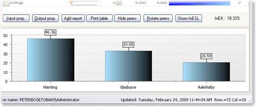
Show peers

· The Peers behind a constructed benchmark becomes visible if you press the Show peers button.

· The names and importance of the Peers are depicted.

· You can change the graphics using Rotate Peers.

Eliminate specific peers

A very useful and popular possibility is to click on a Peer.

· This will eliminate it as a potential peer and the benchmark will change.

· This is a useful way to introduce any soft and subjective information you may have. You may for example know that the data from a given unit is uncertain or that is run using a different management philosophy that cannot or will not be imitated by MyUnit.

· If you are interested to see more details of the Peers Units before deciding to eliminate any, you get full details from the Peer Units tab.

· The eliminated Peers can be reintroduced by using Undo picking in Select Units: Potential Peers tab.

· If you continue to eliminate Peers you will reach a point where no improvements are possible. When this happens, the Benchmark will show how much of extra resources are needed or how much of services we have to give up compared to the best practice of the remaining units.

· If you continue to eliminate Peers you may also reach a point where no comparisons are possible.

InEfficiency Step Ladder

Instead of eliminating Peers one at a time you can also do this in an automated ways by pressing the Inefficiency Step Ladder button InESL. This will initiate a process of successive elimination of the most influential Peer until no further comparisons are possible. The Inefficiency will decline as we eliminate more and more Peers. The resulting levels of inefficiency are depicted in a step function.

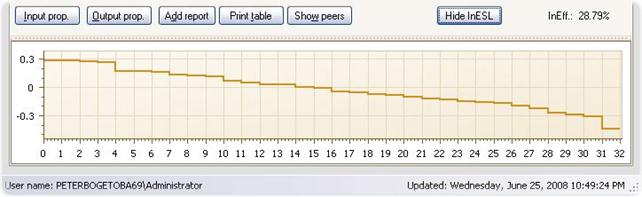
The InESL is useful among others to understand the robustness of estimated improvement potentials. If the InESL function is steep, i.e. declines fast, then the elimination of just a few Peers units may dramatically lower the estimated potentials and therefore the initial estimate relies more heavily on the quality of the fist Peers. If on the other hand the InESL function is flat, the evaluations are not too dependent on exactly which units we can compare to.

The sequences in which units are eliminated are determined by the weight as seen in a usual Shows Peers illustration. At each stage, Interactive Benchmarking IB^® eliminates the Peer with the highest weight and then recalculate the improvement potentials.

Scale (and estimation principle)

The assumed Return to scale and estimation principle can be changed at upper right pull down window.

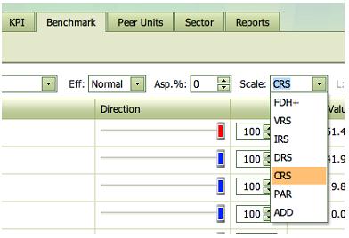
The FDH+, VRS, IRS, DRS, CRS and ADD options are based on so-called non-parametric models (FDH and DEA) models while the PAR option is based on so-called parametric specifications (SFA, Econometrics). The former is based on the idea of minimal extrapolation while the latter is focusing on separation of noise and inefficiency.

The four classical non-parametric specifications make the following assumptions about the return to scale properties:

· Constant Return to Scale (CRS) means that we do not believe there to be significant disadvantage of being small or large

· Decreasing Return to Scale (DRS) means that there may be disadvantages of being large but no disadvantages of being small

· Increasing Return to Scale (IRS) means that there may be disadvantages of being small but no disadvantages of being large

· Variable Return to Scale (VRS) means that there are likely disadvantages of being to too small and too large.

The FDH+ specification allows any pattern of advantages and disadvantages of becoming larger. There may for example be advantages for small units, disadvantages for intermediate units and the again advantages for large units. The FDH approach relies entirely on data to find the properties.

However, when FDH is activated, it becomes possible to make additional assumptions about local constant return to scale. This explains the name FDH+. The idea is that if some entity (Unit) has used certain inputs to produce certain outputs, then we could also proportionally scale inputs and outputs with any factor in the interval from L to U. Traditional FDH therefore is the special case where L=U=1.

The ADD specification is based on the assumption that one can always repeat what others have done. One can therefore create a firm by adding any number of other firms since the logic is that one can always organize a large firm as a series of independent small firms. Again ADD allow for many combinations of advantages and disadvantages of being small and large, but there are logical limits to how disadvantaged one can be as a large entity. ADD is also sometimes called FRH= Free Replicability Hull. For details, see Bogetoft, P. and L. Otto, Benchmarking with DEA, SFA, and R, Springer 2011

The return to scale properties of PAR depends entirely on the properties of the underlying parametric form. In general however it is more restricted that the DEA specification and certainly more restricted than the FDH specification.

For more on the Return to Scale, press here.

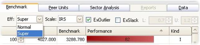
Efficiency

Another control is the Efficiency. There are two possible settings for this.

· Normal efficiency means that the evaluated unit can be compared to itself. In that case, it is always possible for find a benchmark at least as good as the MyUnit.

· Super efficiency means that the evaluated unit cannot be compared to itself. In that case, we are comparing with the best practice of others only. If MyUnit is not a best practice unit, the two calculations coincide. If MyUint is a best practice unit, however, it will usually not be possible to find a benchmark at least as good as the MyUnit. In such cases, the Benchmark may use more of some input or produce less of some outputs. The interpretation is that these are the increases in resource usage and the reductions of service provisions that MyUnit could introduce without loosing its status as a best practice unit.

Super efficiency is hereby a more informative measure than Normal efficiency. Moreover, it is notion very useful in for example performance based payment schemes.

Note: In the next version of the program, we will also extend the Efficiency choices to include fractiles or quantiles. The idea will be to find benchmarks that are 10% from best practice, 20% from best practice etc. This will allow the user more flexibility in setting the ambition level in the benchmarking.

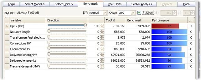
Exclude slack

The Benchmark calculated gives the maximal possibilities to improve MyUnit in the Improvement Direction chosen. In addition to improvements in the proportions specified by the Direction, there may be possibilities to make individual improvements, i.e. improvements in some of the dimensions but not in all of the directions. The see the extra potentials to improve in the directions, you can tick the ExSlack box. This will if possible determine a new benchmark that uses the same or fewer inputs and produces the same of fewer outputs than the original benchmark.

Exclude outliers

If the analyses of a pre-defined model suggest that some of the observations are likely outliers, the likely outliers for the given model can be listed in the data file. When calculating the Benchmark, the user can then choose if he wants to exclude or include the likely outliers. The default setting is that potential outliers are excluded, and the ExOutliers check box is therefore checked by default.

Aspiration

The aspiration Asp.% pull down allow user to benchmark against performance standards that are x% above or below best realized practice.

If for example the aspiration level is set to -10%, it means that we strive only to be 10% below the best practice production frontier. This is also useful to take into account expected productivity improvement, eg a 2% percent improvement in productivity over the next year can be accounted for by contemplating a 2% aspiration level based on today’s data.

The aspiration level is in absolute terms. If user’s aspiration is to be for example among the 10% best performing firms, a sector analysis can be done based on an output proportional direction, and the top 10% fractile of the efficiency distribution can be read off the distribution graph. If this is for example 1.17, it means that an absolute aspiration level of 17% corresponds to the top 10% performance.

The aspiration level has no impact in models without any outputs.

Merger analysis

The Merger analysis button activates a merger analysis module in a pop-up window. It estimates the potential gains from a merger and decomposes these into learning, harmony and size effects.

The analysis concerns a hypothetical merger of MyUnit, as indicated at the top left of the screen, and a merger candidate as specified in the Merge with drop down box of the Merger analysis window. It is therefore easy to change which merger to analyze.

The decomposition of gains can be done in different directions, viz input based and multiplicative, output based and multiplicative, as well as directional and additively, where the direction is as specified by user in the Benchmarking tab.

The general interpretation is however the same:

· Total_E is the total potential gains from a merger and it measures the total possibilities to improve a firm that runs like if it has two divisions with the inputs and outputs of MyUnit and the merger candidate, respectively.

· Pure_Estar is the potential gains when the possibilities to make individual improvements in the merging parties have been eliminated. It therefore represent the potential gains from a collaboration that extends beyond the sharing of best practice ideas

· Learning_LE measures what can be gained if the merger parties individually learn best practices. It is the learning effect that is eliminated when going from total potential gains to the pure merger gains.

· Harmony_HA or mix effect measures what can be gained if the merging parties shared resources (inputs) and obligations (outputs) but remained independent entities. It measures what can be gained if the merging parties reallocated inputs and outputs between them. To activate the harmony (mix) effect, one basically must allow binding contracts between the merging parties.

· Size_SI effect measures the gains or losses from having a merged firm that is larger than the firms merging

The interpretation moreover depends on the direction

· Input multiplicative. Here 1- Values represent a gain. Thus for example, HA=.8 means that by reallocating inputs and outputs, there is a 1-0.8=20% potential to save inputs while keeping the outputs unaffected. Similarly, SI=1.2 means that there is a 1-1.2=-20% gain, i.e. a 20% loss, from having to operate the merged firm at a larger scale.

· Output multiplicative. Here Value-1 represents a gain. Thus for example, HA=1.3 means all outputs could have been expanded with 30% without spending more inputs, if inputs and outputs where reallocated between the two parties.

· Directional Additive. Here we measure improvements in bundles of inputs and outputs. One bundle corresponds to the inputs used and the outputs produced in the merging parties and multiplied by the directional weights. Again, a positive value represents a gain and a negative value represent a loss.

The multiplicative decompositions is

E= LE * Estar = LE * HA * SI

while the additive decompositions means that

E = LE + Estar = LE + HA + SI

The details of the decomposition is described in

Bogetoft, P., Efficiency Gains from Mergers in the Health Care Sector, Part B: Modelling and Part C: Implementation, Research Papers 2008:07 and 2008:08, NZa, The Netherlands.

Bogetoft, P. and D. Wang, Estimating the Potential Gains from Mergers, Journal of Productivity Analysis, 23, pp. 145-171, 2005

Bogetoft, P. and L. Otto, Benchmarking with DEA, SFA, and R, Springer 2011

Add report

When you have an interesting benchmark, you can make a report to remember the comparisons and to produce a nice report of your findings. The Add report feature can be used repeatedly changing for example the direction or the return to scale assumptions in the Benchmark tab. You can also change the Model or the Unit to see comparisons from an alternative perspective or for another entity.

Once we have added at least one report, the Error! Reference source not found. tab becomes active. It keeps the reports on stock for later printing or editing in the Reports tab.

Print table

You can also print the comparison table by pressing Print table. This produces a snap short picture that can be saved as a pdf file.

Peer Units

Peer Units

The Peer Units tab provides additional information about the calculated Benchmark. You get

· The names of the Peer units

· Their relative importance (weights sum to 100)

Peer graphics

The upper pie or graph illustrates the relative importance of the Peers units. You can cycle between alternative illustrations by simply clicking on the illustration

Additional Peer information

The lower window show

· Any additional information available about the units are shown in the lower window.

· Besides the inputs and outputs behind the calculations, this includes all the “Read-only” and “Locked” information from the data set, see also Select Model: Selfdefined Model

Use of additional information

The additional information is useful to guide and refine in an iterative process the

· Filtering in the Select Units: Potential Peers tab

· Individual picking (elimination) of Peers in the Benchmark tab

· Focus or model in the Select Model: Selfdefined Model tab. You may for example focus one some process model where a Peer might do particularly well.

Depending on the data available, it may also give

· Easy contact and further information links, e.g. to the Peer units homepage, its phone number, the names of the CEO, CFO etc.

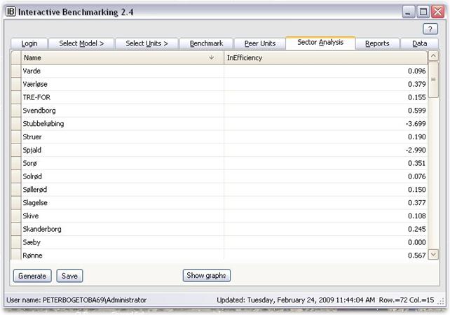
Sector Analysis

Sector Analysis

In the Sector Analysis tab, you can

· Generate the inefficiencies for all the Units in the Sector under some common presumptions.

· Save the results in an Excel file

· Illustrate the results in four different Graph types Density, Distribution , Impact and Second stage, with additional individual options

The Inefficiency Scores

The inefficiency scores reported are the delta inefficiencies.

· They measure the number of times MyUnit could save the input vector and expand the output vector.

· Large values therefore indicate inefficiencies

Presumptions

· The evaluations are done in the Direction (%s) chosen in the Benchmark tab.

· The calculations are relative to the technology used in the Benchmark tab

Saving and illustrating the results

The results can be save as an Excel file for further illustrations and analyses using other tools

Graphs

Also, IB offers four possibilities to illustrate the results, namely

· Density

· Distribution

· Impact

· Second stage

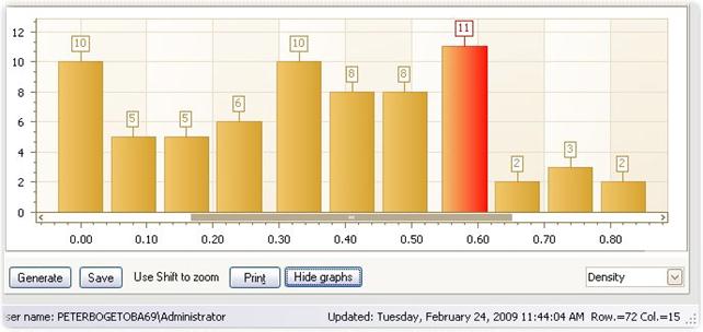
Density

This is a usual histogram of the delta-efficiencies.

· You can adjust then number of grouping in the density graph.

· By clicking on one of the bars, you get the list of Units with corresponding delta-efficiencies.

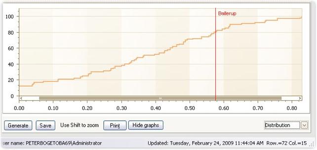
Distribution

This is a usual cumulative distribution of the inefficiencies.

· The unit focused on, MyUnit, is marked by the horizontal (fractile) and vertical (value) lines.

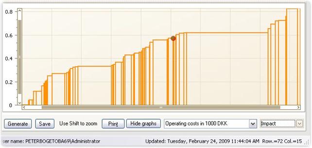
Impact

The Impact graph shows the delta-inefficiencies on the vertical axes and the units on the horizontal axis.

· Each column represents a Unit.

· The width of the column is proportional to the factor indicated.

· This factor can be changed using the pull-down handle.

· The unit focused on, MyUnit, is marked by a red bullet in the corresponding column.

· Note: This is useful to get an idea of Sector looses since in-efficiency in large units will be represented by wider bars. In this way the area becomes proportional to social losses.

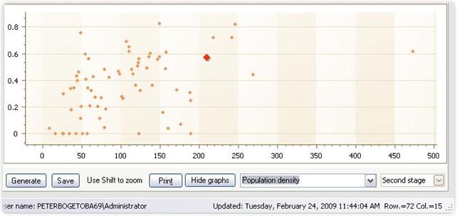
Second stage

The second stage graphs plots the inefficiencies against other variable available.

· You can choose which variable to plot against.

· The plot gives an idea of omitted variables that may have a systematic impact on inefficiency.

· It can be used to (roughly) correct the inefficiencies for such omissions

Zoom and dragging

The graphs in the Sector tab can be examined in more details by scrolling and zooming.

The user can scroll the mouse wheel to zoom in and out of a chart's diagram in the same way one can zoom in commonly used Windows applications.

To activate the zoom function and make the selection more precise, simply press the SHIFT key. The mouse pointer is changed to a magnifying glass. Now select a region on a chart using the left mouse button.

Once the graph has been zoomed, a user can also click a chart's diagram and drag it left and right and up and down by using the hand symbol

Sector reports

You can collect interesting results using the Report facility. A pop-up window is hereby activated in which user can name the report and decide which part of Sector analysis you want to save. New interesting sector results can later be placed in a new Sector report or added to an existing one.

The report can at any time be shown and downloaded in different formats in the Reports tab.

Generate Peers

The Peers of all entities in a DEA or FDH analysis can be generated and displayed in the Sector table by checking the Generate Peers box.

Dynamic

The Dynamic tab allows analysis of performance changes over time.

The tree indices

If the data set contains data from different periods, the Dynamic tab allows user to calculate the Malmquist productivity measure, in IB simple called Total Effects, and its decomposition into Catch-Up and Frontier-Shifts elements. The interpretations of the measures are as follows:

Total effect is the total performance improvement from one period to the next. A value of 1.1 suggests that the entity has increased outputs per input with 10% compared to last period.

Catch-Up is the improvement from one period to the next comapraed to best practice, i.e. a value of for example 1.1 suggest that the entity has improved its performance compared with best practice with 10%. It has in other words not only been able to follow the changes of the best practice enties, it has been catching up upon these.

Frontier shift is the improvement of best practice from one period to the next. A value of 1.2 for example means that it has become possible to reduce inputs with 20% or to expand outputs with 20%.

Note that

Total Effect = CatchUp x FrontierShift.

i.e. Total Effect is a product of the CatchUp and FrontierShift effects. If the best companies for example lowers their ability to produce outputs from given inputs with 10% and MyUnit improves only 5% compared to the best, the Total Effect is 1.05x0.9=0.945 with the interpretation that MyUnit effectively has become 5.5% less productive. If on the other hand a firm has increased its services with 20% compared to best practices, and if best practices has improved by 10%, the firm has actually improved with a factor 1.2x1.1 = 1.32, i.e. it has improved with 32%.

Tables and graphs

The table and illustrations gives the measures for the analyzed unit, MyUnit, as well as average values of the different measures across all entities.

User can chose which DEA model to use in the calculations, which unit to display separately, as well as whether to use output or input based measures

User can also change the type of graphical illustration and the Color scheme used in these.

In addition to studying changes over time, Dynamic analysis can also be used to study frontier shift and catch-up effects related to other differences in the way the entities operate. Instead of time, user data can be divided according to for example firm nationality or ownership structure to get an evaluation of the impact of moving from one country to another or from one ownership type to another.

The formula

Let us close with a more precise and formal definitions:

In the scientific literature, productivity refers to changes over time. If outputs change more than inputs, productivity improves. The standard approach to dynamic evaluations is to use the Malmquist indices. They measure the change from one period to the next by the geometric mean of the performance change relative to the past and present technology.

Specifically, let E_i(s,t) be a measure of the performance of Firm i in period s against the technology in period t. Hence, it could be the measure of proportional input reductions possible or the inverse of the measure of proportional output expansions.

Now, Firm i’s improvement from period s to period t can be evaluated by the Malmquist index M_i(s,t) given by

The intuition of this index runs as follows. We seek to compare the performance in period s to period t. The base technology can be either the s or t technology, so we take geometric mean. Improvements make nominator larger than denominator. Hence, M > 1 corresponds to progress and for example M = 1.2 would suggest a 20% improvement from period s to t, i.e. a fall in the resource usage of 20%.

The change in performance captured by the Malmquist index may be due to two, possibly enforcing and possibly counteracting factors. One is the technical change, TC, that measures the shift in the production frontiers corresponding to a technological progress or regress. The other is the efficiency change EC that measures the catch-up relative to a fixed frontier. This decomposition is developed by a simple rewrite of the Malmquist formula above given by

Again the interpretation is that values of TC above 1 represent technological progress – more can be produces using less resources – while values of EC above 1 represents catching-up, i.e. less waste compared to the best practice of the year.

The Malmquist measure and its decomposition is useful to capture the dynamic developments from one period to the next. Over several periods, one should be careful in the interpretation. One cannot simply accumulate the changes since the index does not satisfy the so-called circular test, i.e. we may not have M(1,2) x M(2,3) = M(1,3) unless the technical change is so-called Hicks-neutral. This drawback is shared by may other indices and can be remedies by for example using a fixed base technology.

Reports

The Reports tab contains references to the Reports generated in the Benchmark tab. The Reports are named by default in accordance with the calendar time when they were generated.

Report formats

The font used in the reports can be changed using any available fonts in the Windows system.

Also once opened, a report can be saved in different formats; this allows you to make final reports in PDF format right away as well as to save the reports in editable formats like HTLM, MHT, RTF, Excell, CSV, Text and Image.

Last but not least, user can choose the report language. Version 2.4 supports English and Danish reports.

Report content

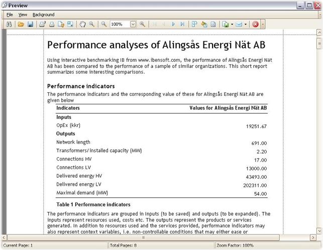
The automatically generated benchmarking reports are written as self-contained reports. The information they contain include:

· MyUnit

· Performance indicators used

· Performance objectives (direction)

· Benchmark with and without slack

· Aggregate Inefficiency index

· Peer units and relative importance of these (where relevant)

· Robustness of evaluations (InESL)

· Model assumptions

· Details about actual Peers

· Brief remarks about Interactive Benchmarking IB^®

The typical size of a report is 9-12 pages.

The reports are automatically adjusted to reflect the specific context (Model, Unit etc).

The KPI and Sector reports are more basic.

Data: Data

Data

The Data sub-tab contains the (raw) data that are used by the program. A data set gives the for each unit its

· DMU (a number assigned for easy reference)

· Names of the Units

· Variables

In IB-Web, you can store multiple data sets and choose which one to analyze by pressing the associated green arrow. You can also download data sets and delete them.

Load new set of data in IB-Win

It is possible to load a new data set using the Load new data push button.

· The new data must be in an Excel Spreadsheet and be properly formatted.

· If a new data set is successfully loaded the program returns to the login page and a usual IB session can begin

Load new set of data in IB-Web

It is possible to load a new data set using one of two methods in IB-Web.

Method 1 let you upload a pre-specified xls work-book. Such data sets must be given as Excel Spreadsheet and be properly formatted.

Method 2 allows you to define a data set on the fly without having to know how to format the xls work-book pages. Creating a new data set this way will guide the user through the necessary steps.

Before a new data set can be directly loaded, it must be properly formatted

Preparing a new data set

Before a new data set can be directly loaded, it must be properly formatted.

The new data must be formated in Excel with up to 7 sheets:

· DMUData

· ModelData

· Scenario/Survey

· LoginInf

· Sponsor

· Outliers

· PeerGroups

· Vtrans

· Storytelling

· Format

· PARData

To prepare a new data file, take a look at the content of the test data.

DMUData

· In DMUData we need unit number, unit name and then all variables in the columns

· It does not matter if you use comma or full stops as decimal point

· In DMUData sheet, all variable columns must be formatted as numbers (i.e. mark cells, right click, and in number tab mark number (as opposed to for example currency or date). The DMU and Name columns are formatted as “General”.

ModelData

· In ModelData we need similar info. No is model number, DefaltCalcType is return to scale (FDH, CRS, CRS, DRS, IRS), Name is a model name that will show up in the Select Model: Predefined Model tab, and Description is the text that comes with the model. The remaining columns are the variables. They must be defined as I (input), O (output), R (read-only) and Locked (any variable) to fully define the model., se also the Select Model: Selfdefined Model.

· In ModelData, use Text to format columns except the Description column where you use General

Scenario / Survey

Scenario / Survey in IB-Web is defined by introducing a tab named Scenario in the Data work book. If there is no such tabs in the data file, there will be no Scenario / Survey tab in the IB Web system that a user is using. Scenarios / Surveys are affiliated with models and must therefore be numbered. Scenario_1 relate to model 1, Scenario_2 to model 2 etc.

An example of a Survey dab in the xls file together with the survey page as it will present itself in the IB-Web system is shown below. We see that there two models with Scenarios/ Surveys (Scenario_1 and Scenario_2. The data generated in connection with the definition of a new unit in model 1 is stored in Scenario_1_11 since the new unit becomes number 11 in the DMUData sheet.

In the definition of the basic Scenario / Survey, as in the first picture, the column headings are fixed and define the following

· ID numbers the questions

· Question column contains first the text that will be shown a heading in the user’s screen, and next the formulation of the questions that a user will meet

· Variable name column define the variable names of the Results associated with the different Questions. These are the names used internally in the program and used also if the user chooses to Self-define a model.

· Answer1,… columns are where the user shall provide answers. The heading shown to the user is given in the second row, and the user can fill in values in the corresponding cells. If a user shall not fill in a number, the cell can he removed by the code [hide]. Surveyor can choose the number of Answer columns freely.

· Result column contains first a heading and next a definition of derived values that will be shown to the user when he updates the Survey page. Any xls formula can be used to define these values. The Result column values are the values that are assigned to the corresponding variables listed in the Variable name column and which are used in the program.

· NewVariable1,… columns allow Surveyor to define other derived values that can be used in the models. The derived value will be assigned to variables with names as given in the second row, and the formulas for calculating the values are given in the third row.

· Notification column is used to define data validation rules. logical tests based on some of the submitted or derived values are usually introduced as illustrated in the example. Warning texts are displayed in red.

· Description column contains in the second row the initial text that will be shown on the screen before the questions

· Remark column contains in the second row a text that will be displayed after the questions.

· Provider email gives the email of the provider (surveyor) to whom an email will be send every time the user Sends new information.

The values that can be used in the benchmarking are the values named in the NewVariable1, NewVariable2 columns and in the Variable name column. To use them they must be introduced in the Data and the Model tabs as illustrated in the second figure above, where we have saved values for Center 1 and Center 1 with alt. cost allocation. They are introduced here by the direct user activating the Save button.

When the direct user Sends data, the survey provider gets an email notification from interactivebenchmarking@gmail.com titled Survey done! with a link from which Provider can collect the new data.

In addition to the core data submitted, i.e. the Answer1, Answer2,.. column information, the sheet also contains information about who has provided the information and which unit they refer to. An example is shown below. We see that data has last been send by User named peter and that it refers to Unit called Center 7.

LoginInfo

· In LoginInfo, you can choose to insert no information. This will give you full flexibility and will allow you to start the program without a login username and a password.

· Alternatively, the Login consisted of users, passwords and indicators of their access rights levels (1,..,10).

· The access rights level determines what the program will show, i.e. which tabs and sub-tabs (and windows) will be available to the specific user.

Sponsor

The Sponsor sheet contains information Name, i.e. a prename to Interactive Benchmarking, e.g. “Water” that will appear in blue about Interactve Bencmarking at the Login tab.

Also the sheet contains information about URL of the sponsor.

Outliers

The outlier tab allows you to specificy for each model a set of potential outliers. The first row contains the model name and the potential outliers of the corresponding model are listed using the Units’ Names below.

When ExOutlier in Checked in Benchmark tab, all calculation are done with the outliers excluded, i.e. they are not allowed to influence the best practice frontier. In the example below, we exclude in the model named Distr. D&V Model 1x4 only one Unit, namely “Aabenraa Forsyning Service A/S”, while in the model Distr. Total Cost Model 2x4 we exclude also “Grindsted Vandværk A.m.b.a.”

PeerGroups

Potential Peer groups can not only be define during a session. They can also be pre-specified by introducing tab in the Data work book called PeerGroups. A group is given a name in the first row, and the Units in the group will be listed using their Names in the rows below. In the KPI and Benchmarking tabs, the user can then scrool down the list of defined Peer Groups to find one that is particularly relevant. In the example below, we have in the second column defined a PeerGroup call Frederiksberg Municipality and consting of the schools named Lindevangskolen, Søndermarkskolen,…, Skolen ved Søerne

A more advanced type of Peer Groups are the ConditionalPeerGroups. They are defined by R scripts. Hereby the user can define Peer Groups that among other things depend on the individual unit, MyUnit being analyzed. Such Peer Groups come with the special attached sign in the program as shown below

To define R scrip based peer groups, the user most introduce a tab called PeerGroupConditions as in the example below.

In this example, two R based Peer Groups are defined. Group 2 is a simple one consiting of Units 1, 3, 4 and 7, while the Group 4 is more complicated and derived from a genuine R loop. The rules for generating R based Conditional Peer Groups are:

As inputs to the R based procedure one can use

ib_DMUData = a matrix with data exactly like the data in the DMUData tab of the xls sheet.

ib_MyUnit = the DMU number of My Unit

ib_RTS = the return to scale used on the model

ib_benchmarkDirection = the direction in input-output space in which IB searches for benchmark

Notes also that ib_InputNames = names of the inputs in the model and ib_OutputNames = names of the outputs in the model can be accessed as

ib_InputNames<-colnames(ib_selectedInputs)

ib_OutputNames<-colnames(ib_selectedOutputs)

As output one most generate

Ib_UserConditionalPeers = a list (vector) of the DMU numbers that shall constitute the Peer Group for the given ib_MyUnit.

As an example of code, assume that we have data from several years and are interested to use the 2010 frontier. We also want to exclude firms that are frontier outliers as defined by the criteria used in German regulation by BNetzA. The script could then read:

# WE INITIALLY DEFINE

ib_InputNames<-colnames(ib_selectedInputs)

ib_OutputNames<-colnames(ib_selectedOutputs)

# FIRST SET OF FILTER

full_data <- complete.cases(ib_DMUData[,c(ib_InputNames,ib_OutputNames)])

correct_year <- (ib_DMUData[,"Year"]==2010)

active_dmus <- (full_data*correct_year==1)

# OUTLIER BASED FILTER THE BNETZA STANDARD

# PREPARATION

library(Benchmarking)

ib_MatrixDirection <- as.matrix(ib_DMUData[active_dmus,c(ib_InputNames,ib_OutputNames)]) %*% diag(ib_benchmarkDirection)

ib_inputMatrix <- ib_DMUData[active_dmus,ib_InputNames,drop=FALSE]

ib_outputMatrix <- ib_DMUData[active_dmus,ib_OutputNames,drop=FALSE]

ib_NumberActiveDMU <- dim(ib_inputMatrix)[1]

# SUPER EFFICIENCY OUTLIERS q_OUTLIER

ib_SuperResults<-sdea(ib_DMUData[active_dmus,ib_InputNames], ib_DMUData[active_dmus,ib_OutputNames], ib_RTS, ORIENTATION="in-out",DIRECT=ib_MatrixDirection)

q=as.matrix(quantile(1-ib_SuperResults$eff))

q_extreme <- q[4,1]+1.5*(q[4,1]-q[2,1])

q_outlier <-ifelse((1-ib_SuperResults$eff)>q_extreme,1,0)

# F TEST BASED OUTLIERS F_outlier

B=dea(ib_inputMatrix, ib_outputMatrix, ib_RTS, ORIENTATION="in-out",DIRECT=ib_MatrixDirection)$eff

F_test =NULL

for ( i in 1:ib_NumberActiveDMU) {

A <- dea(ib_inputMatrix[-i,,drop=FALSE],ib_outputMatrix[-i,,drop=FALSE],RTS = ib_RTS,ORIENTATION="in-out",DIRECT=ib_MatrixDirection[-i,])$eff

SS1=t(A)%*%(A)

SS2=t(B[-i])%*%(B[-i])

C <- pf(SS1/SS2, ib_NumberActiveDMU-1,ib_NumberActiveDMU-1)

F_test <-rbind(F_test,C)

}

Prob_F_test <- F_test[,1]

F_outlier <- (Prob_F_test<0.05)

# THE FINAL SET OF CONDITONAL PEERS

ib_UserConditionalPeers <- setdiff(ib_DMUData[active_dmus,"DMU"]*(1-q_outlier)*(1-F_outlier),0)

For more on R codes, see www.r-project.org

Variable transformation Vtrans

Relevant variable transformations can be defined using R codes in a Vtrans sheet. In a school example where we define three different ways to present final grades this sheet may look as follows:

Each column defines a new variable transformation. The name of the transformation as it will show up in the MyUnit tab is given in the first row. The R code defining the transformation is given is the second row.

As inputs to the R based procedure one can like in Conditional Peers Groups use

ib_DMUData = a matrix with data exactly like the data in the DMUData tab of the xls sheet.

ib_MyUnit = the DMU number of My Unit

As output one most generate a new data set

Ib_NewDMUData

that will then serve as the basis for the subsequent calculations.

For more on R codes, see www.r-project.org

Storytelling

· Storytelling

Dynamic data

To allow dynamic data analysis, i.e. changes over time, IB need data on the entities performance from two or more periods.

The Dynamics tab automatically becomes available when the underlying data set has multiple versions of DMUData, namely the normal tab called DMUData and one or more alternative DMU data tabs called DMUData-1, DMUData-2, etc. In addition, the data file should have a tab called Dynamic with information which periods are at stake and shall be displayed.

The columns in the data sets DMUData, DMUData-1, DMUData-2 etc shall be the same, but this is really no restriction since different entities may have no-available data in different periods.

The rows, i.e. the entities does not need to be the same.

IB will automatically for each pair of periods determine which entities have the necessary data, and it will calculate the measures based on these.

Peer Groups used in the calculations are taken from the Benchmark tab.

Format

It is possible to partially control the format of the numbers as they are displayed in the IB. This is done by introducing a tab in the xls sheet called Format.

One can use a Common format, by introducing a Column with heading Common, or one can use formats that varies between the Unit, KPI, Benchmark, PeerUnits and Sector tabs as illustrated below:

The definition of the format codes follow the description in

http://msdn.microsoft.com/en-us/library/dwhawy9k.aspx

F for example stands for fixed points and the number after F defined the number of decimal digits. The use of decimal sign, . or , is determined by the computer in the case of IBWin and by the server in the case of IBWeb. IBWeb presently uses US formats, i.e. “.” as the decimal separator and “,” as the thousand separator if such a one is requested (N2 for example means that we use (N) integral and decimal digits, group separators, and a decimal separator with optional negative sign, and two digits (2)).

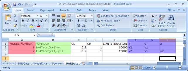
PARData

The PARData sheet contains the parametric form used when PAR is chosen as the estimation method in the Error! Reference source not found. fold-down menu of the Error! Reference source not found. tab.

The data is provides in columns with headings

· MODEL NUMBER

· FORMULA

· GL

· GH

· LIMIT

· Variables short hands

The MODEL NUMBER is a number corresponding to the model numbers used in ModelData sheet.

The FORMULA shall describe the Shepard inputs distance function. Feasible input-output combinations are those with a value of the Shepard inputs distance function larger than or equal to 1, and the frontier corresponds to the Shepard distance being equal to 1.

To determine points on the parametric frontier, Interactive Benchmarking IB^® must solve a possibly complex line search problem. To do so, it uses a so-called bisection method. Trial starting values for this procedure are given by GL and GH, where GL is the change that shall make the solution feasible and GH is an initial value that shall make it infeasible. If this is not the case in reality, IB lowers GL and increases GH to get a feasible starting solution. Once a feasible combination of a point inside and outside the frontier is determined as the starting point, IB performs up to LIMIT bisections. The bisections stops when the difference between the resulting GL and GH values are less than 0.0001.

The Variable short hands are the variables referred to in the FORMULA. In the respective MODEL lines, the corresponding inputs and output names (as used in DMUData) are provided.

Checking a new data set

When a dataset is uploaded, it can be automatically tested if it fulfills a series of the most important requirements. If one of the tables for example have two columns with the same heading, the tables will no pass the Integrity tests and a warning will be issues in the test results.

Data: Models

Models

The Models sub-tab of the Data tab contains the information about the Select Model: Pre-defined Models.

Content

In ModelData you will find the following information for each model:

· No is model number

· DefaltCalcType is Return to scale (CRS, CRS, DRS or IRS),

· Name is the model name that will show up in the Select Model: Predefined Model tab

· Description is (short) explanatory text that comes with the model and that guides the user between the choice of alternative models.

· Variables columns contain the list of variables and an indication of their nature (I, O, R and L)

Variable types

Variables of a given model is classified as

· Inputs (I), i.e. resources and costs used

· Outputs (O), i.e. the products or services generated

· Read-only (R), variables, i.e. variables you could have used as inputs or outputs

· Locked (L), any variable that contain alphanumeric information and that cannot be used as inputs or outputs.

Return to scale

There are six possible settings for the Return to scale:

· Constant Return to Scale (CRS) means that we do not believe there to be significant disadvantage of being small or large

· Decreasing Return to Scale (DRS) means that there may be disadvantages of being large but no disadvantages of being small

· Increasing Return to Scale (IRS) means that there may be disadvantages of being small but no disadvantages of being large

· Variable Return to Scale (VRS) means that there are likely disadvantages of being to too small and too large.

· Extended Free Disposability of Hull (FDH+) is used together with L and H values to suggest no general scale properties but local CRS.

· Additivity (ADD) mean that one can always repeat what others have done, and one can therefore also do what any combination of other have done by letting the parts operate as independent entities

Change content of Data: Model tab

You change the Model data by loading a new data set from the Data:Data tab in IB-Win or from the Data tab in IB-Web.

Data: Setup

Observation: This tab is not available in all versions of Interactive Benchmarking IB^®.

Set-up

The Setup sub-tab of the Data tab allows you to modify a selection of

· Colors

· Fonts

in the different tabs.

Base colors

The base colors are given by the

· Color coordinates 224,224,224

and they can be selected by choosing the first color in the second row of Custom colors when you role down the color selections handles.

If you want to keep the color setting, you must Save them. They will then be the starting colors next time to load IB unless an update of the program is received from the provider.

Base font

The base font is given by

· Xxxx

and you can choose your preferred font from the Change font pup-up window.

If you want to keep the font setting, you must Save it They will then be the starting font next time to load IB unless an update of the program is received from the provider.